Tutorial 1: A basic introduction to pysumma functionality

This notebook gives a brief overview of pysumma functions.

It was originally created by Bart Nijssen and Andrew Bennett (University of Washington) for the “CUAHSI Virtual University snow modeling course 2019”. Modifications include a change of data and update of the naming scheme to comply with SUMMA v3.0. Source: https://github.com/bartnijssen/cuahsi_vu_2019

Loading the required modules

%pylab inline
%load_ext autoreload
%autoreload 2
%reload_ext autoreload

import pysumma as ps
import pysumma.plotting as psp
import matplotlib.pyplot as plt
!cd data/reynolds && ./install_local_setup.sh && cd -

/home/bzq/workspace/pysumma/tutorial

Instantiating a simulation object

To set up a Simulation object you must supply 2 pieces of information.

First, the SUMMA executable; this could be either the compiled executable on your local machine, or a docker image.

The second piece of information is the path to the file manager, which contains all file paths and names needed for a SUMMA simulation run. To create the Simulation object you can then just pass these to the constructor as shown below.

# Define location of .exe and file manager
executable = 'summa.exe'
file_manager = './data/reynolds/file_manager.txt'

# Create a model instance
s = ps.Simulation(executable, file_manager)

Manipulating the configuration of the simulation object

Most of your interactions with pysumma will be facilitated through this Simulation object, so let’s take some time to look through what is in it. What’s contained in the Simulation object right after instantiation is generally just the input required for a SUMMA run. For a more in depth discussion of what these are see the SUMMA Input page of the documentation. There are several attributes of interest that can be examined. To see each of them you can simply print them. Here’s a very high level overview of what’s available:

• s.manager - the file manager

• s.decisions - the decisions file

• s.output_control - defines what variables to write out

• s.force_file_list - a listing of all of the forcing files to use

• s.local_attributes - describes GRU/HRU attributes (lat, lon, elevation, etc)

• s.global_hru_params - listing of spatially constant local (HRU) parameter values

• s.global_gru_params - listing of spatially constant basin (GRU) parameter values

• s.trial_params - spatially distributed parameter values (will overwrite local_param_info values, can be either HRU or GRU)

Most of these objects have a similar interface defined, with exceptions being local_attributes and parameter_trial. Those two are standard xarray datasets. All others follow the simple API:

print(x)                   # Show the data as SUMMA reads it
x.get_option(NAME)         # Get an option
x.set_option(NAME, VALUE)  # Change an option
x.remove_option(NAME)      # Remove an option

More intuitively, you can use key - value type indexing like dictionaries, dataframes, and datasets:

print(x['key'])    # Get an option
x['key'] = value   # Change an option

File manager

Let’s take a look at what the file manager text file actually contains:

s.manager

controlVersion 'SUMMA_FILE_MANAGER_V3.0.0'
simStartTime '1999-10-01 01:00'
simEndTime '2002-09-30 23:00'
tmZoneInfo 'localTime'
settingsPath '/home/bzq/workspace/pysumma/tutorial/data/reynolds/settings/'
forcingPath '/home/bzq/workspace/pysumma/tutorial/data/reynolds/forcing/'
outputPath '/home/bzq/workspace/pysumma/tutorial/data/reynolds/output/'
decisionsFile 'snow_zDecisions.txt'
outputControlFile 'snow_zOutputControl.txt'
globalHruParamFile 'snow_zLocalParamInfo.txt'
globalGruParamFile 'snow_zBasinParamInfo.txt'
attributeFile 'snow_zLocalAttributes.nc'
trialParamFile 'snow_zParamTrial.nc'
forcingListFile 'forcing_file_list.txt'
initConditionFile 'snow_zInitCond.nc'
outFilePrefix 'reynolds'
vegTableFile 'VEGPARM.TBL'
soilTableFile 'SOILPARM.TBL'
generalTableFile 'GENPARM.TBL'
noahmpTableFile 'MPTABLE.TBL'

These are the file paths and names as the simulation object s knows them. You can compare this to the contents of the file ./pbhm-exercise-2/settings/reynolds/summa_fileManager_reynoldsConstantDecayRate.txt to see that they are identical. For this exercise, we’ll focus on three items: the model decisions or parametrizations, parameter values and output control.

Setting decisions

So, now that we’ve got a handle on what’s available and what you can do with it, let’s actually try some of this out. First let’s just print out our decisions file so we can see what’s in the defaults. Note that this only prints the decisions specified in the decision file (./pbhm-exercise-2/settings/reynolds/summa_zDecisions_reynoldsConstantDecayRate.txt) and not all the model decisions that can be made in SUMMA. For a full overview of modelling decision, see the SUMMA documentation: https://summa.readthedocs.io/en/master/input_output/SUMMA_input/#infile_model_decisions

s.decisions

soilCatTbl ROSETTA ! soil-category dataset
vegeParTbl USGS ! vegetation-category dataset
soilStress NoahType ! choice of function for the soil moisture control on stomatal resistance
stomResist BallBerry ! choice of function for stomatal resistance
num_method itertive ! choice of numerical method
fDerivMeth analytic ! choice of method to calculate flux derivatives
LAI_method monTable ! choice of method to determine LAI and SAI
f_Richards mixdform ! form of Richards equation
groundwatr qTopmodl ! choice of groundwater parameterization
hc_profile pow_prof ! choice of hydraulic conductivity profile
bcUpprTdyn nrg_flux ! type of upper boundary condition for thermodynamics
bcLowrTdyn zeroFlux ! type of lower boundary condition for thermodynamics
bcUpprSoiH liq_flux ! type of upper boundary condition for soil hydrology
bcLowrSoiH zeroFlux ! type of lower boundary condition for soil hydrology
veg_traits CM_QJRMS1988 ! choice of parameterization for vegetation roughness length and displacement height
rootProfil powerLaw ! choice of parameterization for the rooting profile
canopyEmis difTrans ! choice of parameterization for canopy emissivity
snowIncept lightSnow ! choice of parameterization for snow interception
windPrfile logBelowCanopy ! choice of canopy wind profile
astability louisinv ! choice of stability function
canopySrad BeersLaw ! choice of method for canopy shortwave radiation
alb_method varDecay ! choice of albedo representation
compaction anderson ! choice of compaction routine
snowLayers CLM_2010 ! choice of method to combine and sub-divide snow layers
thCondSnow jrdn1991 ! choice of thermal conductivity representation for snow
thCondSoil funcSoilWet ! choice of thermal conductivity representation for soil
spatial_gw localColumn ! choice of method for spatial representation of groundwater
subRouting timeDlay ! choice of method for sub-grid routing
snowDenNew constDens ! choice of method for new snow density

Great, we can see what’s in there. But to be able to change anything we need to know the available options for each decision. Let’s look at how to do that. For arbitrary reasons we will look at the snowIncept option, which describes the parameterization for snow interception in the canopy. First we will get it from the decisions object directly, and then query what it can be changed to, then finally change the value to something else.

# Get just the `snowIncept` option
print(s.decisions['snowIncept'])

# Look at what we can set it to
print(s.decisions['snowIncept'].available_options)

# Change the value
s.decisions['snowIncept'] = 'stickySnow'
print(s.decisions['snowIncept'])

snowIncept    lightSnow            ! choice of parameterization for snow interception
['stickySnow', 'lightSnow']
snowIncept    stickySnow           ! choice of parameterization for snow interception

Changing parameters

Much like the decisions we can manipulate the gloabl_hru_param file. First, let’s look at what’s contained in it:

print(s.global_hru_params)

upperBoundHead            |      -7.5d-1 |      -1.0d+2 |      -1.0d-2
lowerBoundHead            |       0.0000 |      -1.0d+2 |      -1.0d-2
upperBoundTheta           |       0.2004 |       0.1020 |       0.3680
lowerBoundTheta           |       0.1100 |       0.1020 |       0.3680
upperBoundTemp            |     272.1600 |     270.1600 |     280.1600
lowerBoundTemp            |     274.1600 |     270.1600 |     280.1600
tempCritRain              |     273.1600 |     272.1600 |     274.1600
tempRangeTimestep         |       2.0000 |       0.5000 |       5.0000
frozenPrecipMultip        |       1.0000 |       0.5000 |       1.5000
snowfrz_scale             |      50.0000 |      10.0000 |    1000.0000
fixedThermalCond_snow     |       0.3500 |       0.1000 |       1.0000
albedoMax                 |       0.8400 |       0.7000 |       0.9500
albedoMinWinter           |       0.5500 |       0.6000 |       1.0000
albedoMinSpring           |       0.5500 |       0.3000 |       1.0000
albedoMaxVisible          |       0.9500 |       0.7000 |       0.9500
albedoMinVisible          |       0.7500 |       0.5000 |       0.7500
albedoMaxNearIR           |       0.6500 |       0.5000 |       0.7500
albedoMinNearIR           |       0.3000 |       0.1500 |       0.4500
albedoDecayRate           |       1.0d+6 |       1.0d+5 |       5.0d+6
albedoSootLoad            |       0.3000 |       0.1000 |       0.5000
albedoRefresh             |       1.0000 |       1.0000 |      10.0000
radExt_snow               |      20.0000 |      20.0000 |      20.0000
Frad_direct               |       0.7000 |       0.0000 |       1.0000
Frad_vis                  |       0.5000 |       0.0000 |       1.0000
directScale               |       0.0900 |       0.0000 |       0.5000
newSnowDenMin             |     100.0000 |      50.0000 |     100.0000
newSnowDenMult            |     100.0000 |      25.0000 |      75.0000
newSnowDenScal            |       5.0000 |       1.0000 |       5.0000
constSnowDen              |     100.0000 |      50.0000 |     250.0000
newSnowDenAdd             |     109.0000 |      80.0000 |     120.0000
newSnowDenMultTemp        |       6.0000 |       1.0000 |      12.0000
newSnowDenMultWind        |      26.0000 |      16.0000 |      36.0000
newSnowDenMultAnd         |       1.0000 |       1.0000 |       3.0000
newSnowDenBase            |       0.0000 |       0.0000 |       0.0000
densScalGrowth            |       0.0460 |       0.0230 |       0.0920
tempScalGrowth            |       0.0400 |       0.0200 |       0.0600
grainGrowthRate           |       2.7d-6 |       1.0d-6 |       5.0d-6
densScalOvrbdn            |       0.0230 |       0.0115 |       0.0460
tempScalOvrbdn            |       0.0800 |       0.6000 |       1.0000
baseViscosity             |       9.0d+5 |       5.0d+5 |       1.5d+6
Fcapil                    |       0.0600 |       0.0100 |       0.1000
k_snow                    |       0.0150 |       0.0050 |       0.0500
mw_exp                    |       3.0000 |       1.0000 |       5.0000
z0Snow                    |       0.0010 |       0.0010 |      10.0000
z0Soil                    |       0.0100 |       0.0010 |      10.0000
z0Canopy                  |       0.1000 |       0.0010 |      10.0000
zpdFraction               |       0.6500 |       0.5000 |       0.8500
critRichNumber            |       0.2000 |       0.1000 |       1.0000
Louis79_bparam            |       9.4000 |       9.2000 |       9.6000
Louis79_cStar             |       5.3000 |       5.1000 |       5.5000
Mahrt87_eScale            |       1.0000 |       0.5000 |       2.0000
leafExchangeCoeff         |       0.0100 |       0.0010 |       0.1000
windReductionParam        |       0.2800 |       0.0000 |       1.0000
soil_dens_intr            |    2700.0000 |     500.0000 |    4000.0000
thCond_soil               |       5.5000 |       2.9000 |       8.4000
frac_sand                 |       0.1600 |       0.0000 |       1.0000
frac_silt                 |       0.2800 |       0.0000 |       1.0000
frac_clay                 |       0.5600 |       0.0000 |       1.0000
fieldCapacity             |       0.2000 |       0.0000 |       1.0000
theta_mp                  |       0.4010 |       0.3000 |       0.6000
theta_sat                 |       0.5500 |       0.3000 |       0.6000
theta_res                 |       0.1390 |       0.0010 |       0.1000
vGn_alpha                 |      -8.4d-1 |      -1.0d+0 |      -1.0d-2
vGn_n                     |       1.3000 |       1.0000 |       3.0000
mpExp                     |       5.0000 |       1.0000 |      10.0000
wettingFrontSuction       |       0.3000 |       0.1000 |       1.5000
k_soil                    |       7.5d-6 |       1.0d-7 |       1.0d-5
k_macropore               |       0.0010 |       1.0d-7 |       1.0d-5
kAnisotropic              |       1.0000 |       0.0001 |      10.0000
zScale_TOPMODEL           |       2.5000 |       0.1000 |     100.0000
compactedDepth            |       1.0000 |       0.0000 |       1.0000
aquiferScaleFactor        |       0.3500 |       0.1000 |     100.0000
aquiferBaseflowExp        |       2.0000 |       1.0000 |      10.0000
aquiferBaseflowRate       |       2.0000 |       1.0000 |      10.0000
qSurfScale                |      50.0000 |       1.0000 |     100.0000
specificYield             |       0.2000 |       0.1000 |       0.3000
specificStorage           |       1.0d-9 |       1.0d-5 |       1.0d-7
f_impede                  |       2.0000 |       1.0000 |      10.0000
soilIceScale              |       0.1300 |       0.0001 |       1.0000
soilIceCV                 |       0.4500 |       0.1000 |       5.0000
Kc25                      |     296.0770 |     296.0770 |     296.0770
Ko25                      |       0.2961 |       0.2961 |       0.2961
Kc_qFac                   |       2.1000 |       2.1000 |       2.1000
Ko_qFac                   |       1.2000 |       1.2000 |       1.2000
kc_Ha                     |       7.9d+4 |       7.9d+4 |       7.9d+4
ko_Ha                     |       3.6d+4 |       3.6d+4 |       3.6d+4
vcmax25_canopyTop         |      40.0000 |      20.0000 |     100.0000
vcmax_qFac                |       2.4000 |       2.4000 |       2.4000
vcmax_Ha                  |       6.5d+4 |       6.5d+4 |       6.5d+4
vcmax_Hd                  |       2.2d+5 |       1.5d+5 |       1.5d+5
vcmax_Sv                  |     710.0000 |     485.0000 |     485.0000
vcmax_Kn                  |       0.6000 |       0.0000 |       1.2000
jmax25_scale              |       2.0000 |       2.0000 |       2.0000
jmax_Ha                   |       4.4d+4 |       4.4d+4 |       4.4d+4
jmax_Hd                   |       1.5d+5 |       1.5d+5 |       1.5d+5
jmax_Sv                   |     495.0000 |     495.0000 |     495.0000
fractionJ                 |       0.1500 |       0.1500 |       0.1500
quantamYield              |       0.0500 |       0.0500 |       0.0500
vpScaleFactor             |    1500.0000 |    1500.0000 |    1500.0000
cond2photo_slope          |       9.0000 |       1.0000 |      10.0000
minStomatalConductance    |    2000.0000 |    2000.0000 |    2000.0000
winterSAI                 |       1.0000 |       0.0100 |       3.0000
summerLAI                 |       3.0000 |       0.0100 |      10.0000
rootScaleFactor1          |       2.0000 |       1.0000 |      10.0000
rootScaleFactor2          |       5.0000 |       1.0000 |      10.0000
rootingDepth              |       3.0000 |       0.0100 |      10.0000
rootDistExp               |       1.0000 |       0.0100 |       1.0000
plantWiltPsi              |      -1.5d+2 |      -5.0d+2 |       0.0000
soilStressParam           |       5.8000 |       4.3600 |       6.3700
critSoilWilting           |       0.0750 |       0.0000 |       1.0000
critSoilTranspire         |       0.1750 |       0.0000 |       1.0000
critAquiferTranspire      |       0.2000 |       0.1000 |      10.0000
minStomatalResistance     |      50.0000 |      10.0000 |     200.0000
leafDimension             |       0.0400 |       0.0100 |       0.1000
heightCanopyTop           |      20.0000 |       0.0500 |     100.0000
heightCanopyBottom        |       2.0000 |       0.0000 |       5.0000
specificHeatVeg           |     874.0000 |     500.0000 |    1500.0000
maxMassVegetation         |      25.0000 |       1.0000 |      50.0000
throughfallScaleSnow      |       0.5000 |       0.1000 |       0.9000
throughfallScaleRain      |       0.5000 |       0.1000 |       0.9000
refInterceptCapSnow       |       6.6000 |       1.0000 |      10.0000
refInterceptCapRain       |       1.0000 |       0.0100 |       1.0000
snowUnloadingCoeff        |       0.0000 |       0.0000 |       1.5d-6
canopyDrainageCoeff       |       0.0050 |       0.0010 |       0.0100
ratioDrip2Unloading       |       0.4000 |       0.0000 |       1.0000
canopyWettingFactor       |       0.7000 |       0.0000 |       1.0000
canopyWettingExp          |       1.0000 |       0.0000 |       1.0000
minwind                   |       0.1000 |       0.0010 |       1.0000
minstep                   |       1.0000 |       1.0000 |    1800.0000
maxstep                   |    3600.0000 |      60.0000 |    1800.0000
wimplicit                 |       0.0000 |       0.0000 |       1.0000
maxiter                   |     100.0000 |       1.0000 |     100.0000
relConvTol_liquid         |       0.0010 |       1.0d-5 |       0.1000
absConvTol_liquid         |       1.0d-5 |       1.0d-8 |       0.0010
relConvTol_matric         |       1.0d-6 |       1.0d-5 |       0.1000
absConvTol_matric         |       1.0d-6 |       1.0d-8 |       0.0010
relConvTol_energy         |       0.0100 |       1.0d-5 |       0.1000
absConvTol_energy         |       1.0000 |       0.0100 |      10.0000
relConvTol_aquifr         |       1.0000 |       0.0100 |      10.0000
absConvTol_aquifr         |       1.0d-5 |       1.0d-5 |       0.1000
zmin                      |       0.0100 |       0.0050 |       0.1000
zmax                      |       0.0750 |       0.0100 |       0.5000
zminLayer1                |       0.0075 |       0.0075 |       0.0075
zminLayer2                |       0.0100 |       0.0100 |       0.0100
zminLayer3                |       0.0500 |       0.0500 |       0.0500
zminLayer4                |       0.1000 |       0.1000 |       0.1000
zminLayer5                |       0.2500 |       0.2500 |       0.2500
zmaxLayer1_lower          |       0.0500 |       0.0500 |       0.0500
zmaxLayer2_lower          |       0.2000 |       0.2000 |       0.2000
zmaxLayer3_lower          |       0.5000 |       0.5000 |       0.5000
zmaxLayer4_lower          |       1.0000 |       1.0000 |       1.0000
zmaxLayer1_upper          |       0.0300 |       0.0300 |       0.0300
zmaxLayer2_upper          |       0.1500 |       0.1500 |       0.1500
zmaxLayer3_upper          |       0.3000 |       0.3000 |       0.3000
zmaxLayer4_upper          |       0.7500 |       0.7500 |       0.7500
minTempUnloading          |     270.1600 |     260.1600 |     273.1600
minWindUnloading          |       0.0000 |       0.0000 |      10.0000
rateTempUnloading         |       1.9d+5 |       1.0d+5 |       3.0d+5
rateWindUnloading         |       1.6d+5 |       1.0d+5 |       3.0d+5

Yikes, that’s pretty long. Let’s change something for the sake of it:

# Print it
print('old: ' + str(s.global_hru_params['albedoMax']))

# Change the value
s.global_hru_params['albedoMax'] = 0.9
print('new: ' + str(s.global_hru_params['albedoMax']))

old: albedoMax                 |       0.8400 |       0.7000 |       0.9500
new: albedoMax                 |       0.9000 |       0.9000 |       0.9000

Modifying output

And one more, we can also modify what get’s written to output. The output control file represents the options available through columns of numeric values. These numbers represent how to write the output. From the SUMMA documentation (https://summa.readthedocs.io/en/latest/input_output/SUMMA_input/#output-control-file) they are arranged as:

! varName          | outFreq | inst | sum | mean | var | min | max | mode

As before, let’s look at what’s in the output_control by simply printing it out:

print(s.output_control)

nSnow                                | 1 | 0 | 1 | 0 | 0 | 0 | 0 | 0
scalarSWE                            | 1 | 0 | 1 | 0 | 0 | 0 | 0 | 0
scalarSnowDepth                      | 1 | 0 | 1 | 0 | 0 | 0 | 0 | 0
scalarSnowfallTemp                   | 1 | 0 | 1 | 0 | 0 | 0 | 0 | 0
scalarSnowAge                        | 1 | 0 | 1 | 0 | 0 | 0 | 0 | 0
scalarInfiltration                   | 1 | 0 | 1 | 0 | 0 | 0 | 0 | 0
scalarExfiltration                   | 1 | 0 | 1 | 0 | 0 | 0 | 0 | 0
scalarTotalSoilLiq                   | 1 | 0 | 1 | 0 | 0 | 0 | 0 | 0
scalarTotalSoilIce                   | 1 | 0 | 1 | 0 | 0 | 0 | 0 | 0
scalarSurfaceRunoff                  | 1 | 0 | 1 | 0 | 0 | 0 | 0 | 0
scalarSurfaceTemp                    | 1 | 0 | 1 | 0 | 0 | 0 | 0 | 0
scalarSnowSublimation                | 1 | 0 | 1 | 0 | 0 | 0 | 0 | 0
scalarLatHeatTotal                   | 1 | 0 | 1 | 0 | 0 | 0 | 0 | 0
scalarSenHeatTotal                   | 1 | 0 | 1 | 0 | 0 | 0 | 0 | 0
scalarSnowDrainage                   | 1 | 0 | 1 | 0 | 0 | 0 | 0 | 0
scalarRainfall                       | 1 | 0 | 1 | 0 | 0 | 0 | 0 | 0
scalarSnowfall                       | 1 | 0 | 1 | 0 | 0 | 0 | 0 | 0
mLayerVolFracIce                     | 1 | 0 | 1 | 0 | 0 | 0 | 0 | 0
mLayerVolFracLiq                     | 1 | 0 | 1 | 0 | 0 | 0 | 0 | 0
mLayerVolFracWat                     | 1 | 0 | 1 | 0 | 0 | 0 | 0 | 0
mLayerDepth                          | 1 | 0 | 1 | 0 | 0 | 0 | 0 | 0
mLayerTemp                           | 1 | 0 | 1 | 0 | 0 | 0 | 0 | 0
mLayerHeight                         | 1 | 0 | 1 | 0 | 0 | 0 | 0 | 0
iLayerHeight                         | 1 | 0 | 1 | 0 | 0 | 0 | 0 | 0
iLayerNrgFlux                        | 1 | 0 | 1 | 0 | 0 | 0 | 0 | 0
mLayerNrgFlux                        | 1 | 0 | 1 | 0 | 0 | 0 | 0 | 0
mLayerLiqFluxSnow                    | 1 | 0 | 1 | 0 | 0 | 0 | 0 | 0
iLayerLiqFluxSnow                    | 1 | 0 | 1 | 0 | 0 | 0 | 0 | 0
iLayerConductiveFlux                 | 1 | 0 | 1 | 0 | 0 | 0 | 0 | 0
iLayerAdvectiveFlux                  | 1 | 0 | 1 | 0 | 0 | 0 | 0 | 0

Note that SUMMA is pretty flexible in its output. What we see above is a pretty typical output file configuration that contains most of the major state variables and fluxes. For a more complete overview of what you can ask SUMMA to output, see: https://github.com/NCAR/summa/blob/master/build/source/dshare/var_lookup.f90

We can modify values in the existing output_control in a couple of ways:

# Check the settings for one of the output variables
print(s.output_control['scalarInfiltration'])
print(s.output_control['scalarInfiltration'].statistic)

# Change the output statistic from instantaneous to sum
s.output_control['scalarInfiltration'] = [1, 1, 0, 0, 0, 0, 0, 0]
print(s.output_control['scalarInfiltration'])
print(s.output_control['scalarInfiltration'].statistic)

# We could also be more verbose:
s.output_control['scalarInfiltration'] = {
    'period': 1, 'instant': 1, 'sum': 0,
    'mean': 0, 'variance': 0, 'min': 0, 'max': 0
}
print(s.output_control['scalarInfiltration'])
print(s.output_control['scalarInfiltration'].statistic)

scalarInfiltration                   | 1 | 0 | 1 | 0 | 0 | 0 | 0 | 0
instant
scalarInfiltration                   | 1 | 1 | 0 | 0 | 0 | 0 | 0 | 0
sum
scalarInfiltration                   | 1 | 0 | 1 | 0 | 0 | 0 | 0 | 0
instant

Running pysumma and manipulating output

Now that you’ve had an overview of how you can interact with SUMMA configurations through pysumma let’s run a simulation. Before doing so we will reset our Simulation object, which will discard all of the changes we’ve made and load in a clean setup. Alternatively you could simply instantiate a new Simulation object. After running the simulation, we will make sure that it completed successfully by checking the status. With a complete run, we can look at the output simply by using the simulation’s output attribute. It is simply an xarray dataset, which can be manipulated in all of the usual ways.

s.reset()
# Or you could just create a new simulation object like before:
#s = ps.Simulation(executable, file_manager)

Before we run the model, we need to ensure that the output directory specified in the fileManger actually exists. If it doesn’t, SUMMA will notify you of this and abort the simulation.

# module to handle tasks related to files and folders
import os

# Make the output directory if it doesn't exist
print('Current specified output directory: ' + s.manager['outputPath'].value)
if not os.path.exists(s.manager['outputPath'].value):
    os.makedirs(s.manager['outputPath'].value)

Current specified output directory: /home/bzq/workspace/pysumma/tutorial/data/reynolds/output/

Now we can try a model run.

s.run('local', run_suffix='_default') # run_suffix allows you to specify a string that will be added to the output file name. This is very useful to keep track of different experiments
print(s.status)

Success

You should have gotten a 'Success' printed out after running the simulation. For further details about the simulation you can look at the full output log that SUMMA produces by printing out s.stdout. In the event that s.status does not return Success you may wish to inspect this log to diagnose the problem further. s.stderror and s.stdout can provide details about the error.

Plotting

Now that we’ve got some output we can plot some results. Because the output is an xarray DataSet we can use the convenient plotting capabilities provided by xarray.

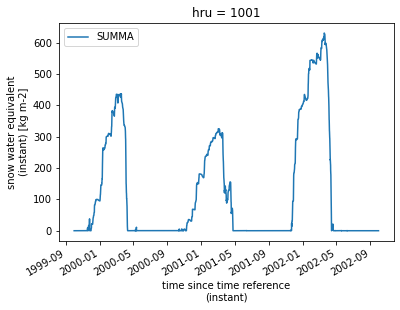
s.output['scalarSWE'].plot(label='SUMMA');
plt.legend(); # note that 'plt' relies on: 'import matplotlib.pyplot as plt' which is magically included in the line `%pylab inline` in the first code block

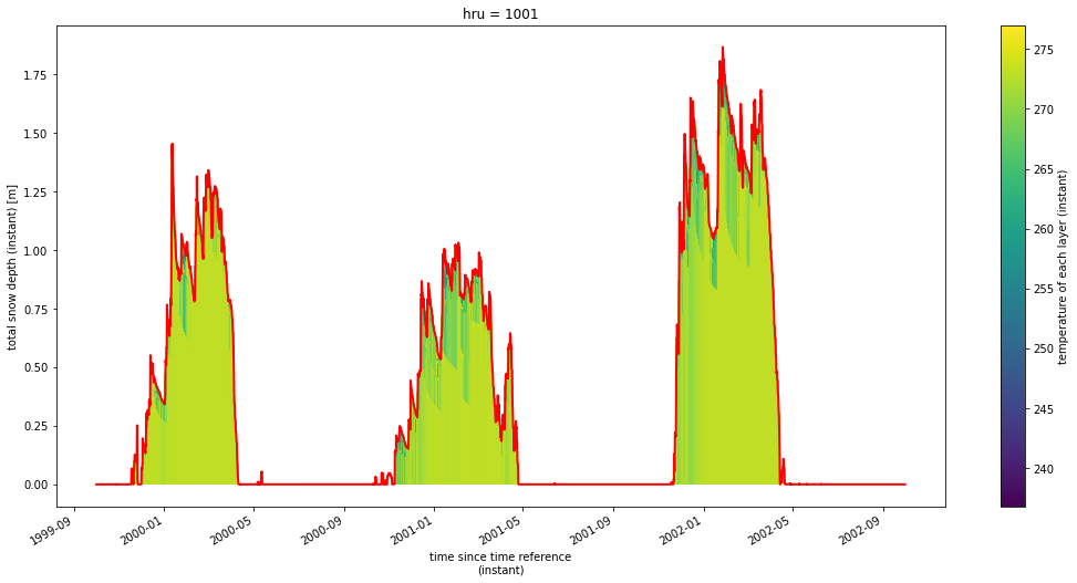
Additionally, pysumma provides some more specialized plotting capabilities. To access it we have the ps.plotting module. First, lets plot the vertical layers over time. For this we will use ps.plotting.layers, which requires two pieces of information. First, the variable that you want to plot. It should have both time and midToto dimensions. The first plot we will make will be the temperature, which uses the variable mLayerTemp, and the second will be the volumetric fraction of water content in each layer, which uses mLayerVolFracWat. To start out we will give these more convenient names.

depth = s.output.isel(hru=0)['iLayerHeight']
temp = s.output.isel(hru=0)['mLayerTemp']
frac_wat = s.output.isel(hru=0)['mLayerVolFracWat']

Now we can plot this using our function. For the temperature plot we will set plot_soil to False so that we only plot the snowpack. We can see that the top layers of the snowpack respond more quickly to the changing air temperature, and that later in the season the warmer air causes temperature transmission to lower layers and ultimately melts out.

psp.layers(temp, depth, colormap='viridis', plot_soil=False, plot_snow=True);
s.output['scalarSnowDepth'].plot(color='red', linewidth=2);

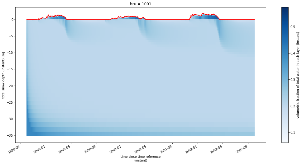
By looking at the volumetric water content we can see even more details. Now we will set plot_soil to True so that we can see how snowmelt can cause water infiltration into the soil. For example, during the melt season in 2012 we can easily see how the snowmelt infiltrates into the ground.

psp.layers(frac_wat, depth, colormap='Blues', plot_soil=True, plot_snow=True);
s.output['scalarSnowDepth'].plot(color='red', linewidth=2);

Tutorial 2: Running ensembles of SUMMA simulations

pysumma offers an Ensemble class which is useful for running multiple simulations with varying options. These options can be parameter values, model structures, different locations made up of different file managers, or combinations of any of these. To demonstrate the Ensemble capabilities we will step through each individually. As usual we will begin with some imports and definition of some global variables.

import numpy as np
import pysumma as ps
import matplotlib.pyplot as plt
from pprint import pprint

!cd data/reynolds && ./install_local_setup.sh && cd -
!cd data/coldeport && ./install_local_setup.sh && cd -

summa_exe = 'summa.exe'
file_manager = './data/coldeport/file_manager.txt'

/home/bzq/workspace/pysumma/tutorial
/home/bzq/workspace/pysumma/tutorial

Changing decisions

The Ensemble object mainly operates by taking configuration dictionaries. These can be defined manually, or can be defined through the use of helper functions which will be described later. For now, we will look at how to run models using different options for the stomResist and soilStress decisions. This is done by providing a dictionary of these mappings inside of a decisions key of the overall configuration. The decisions key is one of several special configuration keys which pysumma knows how to manipulate under the hood. We will explore the others later.

This configuration is used to construct the Ensemble object, which also takes the SUMMA executable, a file manager path, and optionally the num_workers argument. The num_workers argument is used to automatically run these ensemble members in parallel. Here we define it as 2, since that’s how many different runs we will be completing. You can set this to a higher number than your computer has CPU cores, but you won’t likely see any additional speedup by doing so.

We then run the ensemble through the run method which works similarly to the Simulation object. After running the ensemble we check the status by running the summary method. This will return a dictionary outlining any successes or failures of each of the members. In the event of any failures you can later inspect the underlying Simulation objects that are internal to the Ensemble. We will demonstrate how to do this later in the tutorial.

config = {
    'run0': {'decisions':{'stomResist': 'Jarvis',
                          'soilStress': 'NoahType'}},
    'run1': {'decisions':{'stomResist': 'BallBerry',
                          'soilStress': 'CLM_Type'}},
}

decision_ens = ps.Ensemble(summa_exe, config, file_manager, num_workers=2)
decision_ens.run('local')
print(decision_ens.summary())

{'Success': ['run0', 'run1'], 'Error': [], 'Other': []}

We also provide some functionality to make it easier to wrangle the data together via the merge_output method.

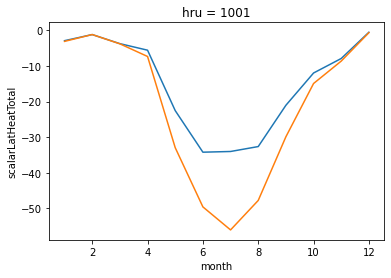
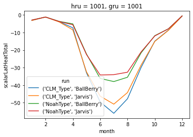
To access the simulations individually you can use the .simulations attribute, which is simply a dictionary of the Simulation objects mapped by the name that’s used to run the simulation. Let’s loop through and print the decisions directly from the Simulation as proof things worked. We can also open the output of each of the simulations as in the previous tutorial, and plot the monthly average latent heat flux for each simulation.

for n, sim in decision_ens.simulations.items():
    print(f'{n} used {sim.decisions["stomResist"].value} for the stomResist option and {sim.decisions["soilStress"].value} for soilStress')

run0 used Jarvis for the stomResist option and NoahType for soilStress
run1 used BallBerry for the stomResist option and CLM_Type for soilStress

run0 = decision_ens.simulations['run0'].output.load()
run1 = decision_ens.simulations['run1'].output.load()

run0['scalarLatHeatTotal'].groupby(run0['time'].dt.month).mean().plot(label='run0')
run1['scalarLatHeatTotal'].groupby(run1['time'].dt.month).mean().plot(label='run1')

[<matplotlib.lines.Line2D at 0x7f8f1a631790>]

Note in the previous example we didn’t run every combination of stomResist and soilStress that we could have. When running multiple configurations it often becomes unwieldy to type out the full configuration that you are attempting to run, so some helper functions have been implemented to make this a bit easier. In the following cell we demonstrate this. You can see that the new output will show we have 4 configurations to run, each with a unique set of decisions. The names are just the

decisions being set, delimited by ++ so that it is easy to keep track of each run.

decisions_to_run = {
    'stomResist': ['Jarvis', 'BallBerry'],
    'soilStress': ['NoahType', 'CLM_Type']
}

config = ps.ensemble.decision_product(decisions_to_run)
pprint(config)

{'++BallBerry++CLM_Type++': {'decisions': {'soilStress': 'CLM_Type',
                                           'stomResist': 'BallBerry'}},
 '++BallBerry++NoahType++': {'decisions': {'soilStress': 'NoahType',
                                           'stomResist': 'BallBerry'}},
 '++Jarvis++CLM_Type++': {'decisions': {'soilStress': 'CLM_Type',
                                        'stomResist': 'Jarvis'}},
 '++Jarvis++NoahType++': {'decisions': {'soilStress': 'NoahType',
                                        'stomResist': 'Jarvis'}}}

decision_ens = ps.Ensemble(summa_exe, config, file_manager, num_workers=4)
decision_ens.run('local')
print(decision_ens.summary())

{'Success': ['++Jarvis++NoahType++', '++Jarvis++CLM_Type++', '++BallBerry++NoahType++', '++BallBerry++CLM_Type++'], 'Error': [], 'Other': []}

When ensembles have been run through these product configurations (we’ll detail a couple others later), you can use a special method to open them in a way that makes the output easier to wrangle. As before we’ll plot the mean monthly latent heat for each of the runs.

ens_ds = decision_ens.merge_output()
ens_ds

<xarray.Dataset>
Dimensions:                (gru: 1, hru: 1, ifcSnow: 6, ifcToto: 15, midToto: 14, soilStress: 2, stomResist: 2, time: 52585)
Coordinates:
  * time                   (time) datetime64[ns] 1994-10-01T00:59:59.99998659...
  * hru                    (hru) int64 1001
  * gru                    (gru) int64 1001
  * stomResist             (stomResist) object 'BallBerry' 'Jarvis'
  * soilStress             (soilStress) object 'CLM_Type' 'NoahType'
Dimensions without coordinates: ifcSnow, ifcToto, midToto
Data variables:
    nSnow                  (time, hru, stomResist, soilStress) int32 dask.array<chunksize=(52585, 1, 1, 2), meta=np.ndarray>
    scalarSnowDepth        (time, hru, stomResist, soilStress) float64 dask.array<chunksize=(52585, 1, 1, 2), meta=np.ndarray>
    scalarSWE              (time, hru, stomResist, soilStress) float64 dask.array<chunksize=(52585, 1, 1, 2), meta=np.ndarray>
    mLayerTemp             (time, midToto, hru, stomResist, soilStress) float64 dask.array<chunksize=(52585, 14, 1, 1, 2), meta=np.ndarray>
    mLayerVolFracIce       (time, midToto, hru, stomResist, soilStress) float64 dask.array<chunksize=(52585, 14, 1, 1, 2), meta=np.ndarray>
    mLayerVolFracLiq       (time, midToto, hru, stomResist, soilStress) float64 dask.array<chunksize=(52585, 14, 1, 1, 2), meta=np.ndarray>
    mLayerVolFracWat       (time, midToto, hru, stomResist, soilStress) float64 dask.array<chunksize=(52585, 14, 1, 1, 2), meta=np.ndarray>
    scalarSurfaceTemp      (time, hru, stomResist, soilStress) float64 dask.array<chunksize=(52585, 1, 1, 2), meta=np.ndarray>
    mLayerDepth            (time, midToto, hru, stomResist, soilStress) float64 dask.array<chunksize=(52585, 14, 1, 1, 2), meta=np.ndarray>
    mLayerHeight           (time, midToto, hru, stomResist, soilStress) float64 dask.array<chunksize=(52585, 14, 1, 1, 2), meta=np.ndarray>
    iLayerHeight           (time, ifcToto, hru, stomResist, soilStress) float64 dask.array<chunksize=(52585, 15, 1, 1, 2), meta=np.ndarray>
    scalarSnowfallTemp     (time, hru, stomResist, soilStress) float64 dask.array<chunksize=(52585, 1, 1, 2), meta=np.ndarray>
    scalarSnowAge          (time, hru, stomResist, soilStress) float64 dask.array<chunksize=(52585, 1, 1, 2), meta=np.ndarray>
    scalarTotalSoilLiq     (time, hru, stomResist, soilStress) float64 dask.array<chunksize=(52585, 1, 1, 2), meta=np.ndarray>
    scalarTotalSoilIce     (time, hru, stomResist, soilStress) float64 dask.array<chunksize=(52585, 1, 1, 2), meta=np.ndarray>
    scalarRainfall         (time, hru, stomResist, soilStress) float64 dask.array<chunksize=(52585, 1, 1, 2), meta=np.ndarray>
    scalarSnowfall         (time, hru, stomResist, soilStress) float64 dask.array<chunksize=(52585, 1, 1, 2), meta=np.ndarray>
    scalarSenHeatTotal     (time, hru, stomResist, soilStress) float64 dask.array<chunksize=(52585, 1, 1, 2), meta=np.ndarray>
    scalarLatHeatTotal     (time, hru, stomResist, soilStress) float64 dask.array<chunksize=(52585, 1, 1, 2), meta=np.ndarray>
    scalarSnowSublimation  (time, hru, stomResist, soilStress) float64 dask.array<chunksize=(52585, 1, 1, 2), meta=np.ndarray>
    iLayerConductiveFlux   (time, ifcToto, hru, stomResist, soilStress) float64 dask.array<chunksize=(52585, 15, 1, 1, 2), meta=np.ndarray>
    iLayerAdvectiveFlux    (time, ifcToto, hru, stomResist, soilStress) float64 dask.array<chunksize=(52585, 15, 1, 1, 2), meta=np.ndarray>
    iLayerNrgFlux          (time, ifcToto, hru, stomResist, soilStress) float64 dask.array<chunksize=(52585, 15, 1, 1, 2), meta=np.ndarray>
    mLayerNrgFlux          (time, midToto, hru, stomResist, soilStress) float64 dask.array<chunksize=(52585, 14, 1, 1, 2), meta=np.ndarray>
    scalarSnowDrainage     (time, hru, stomResist, soilStress) float64 dask.array<chunksize=(52585, 1, 1, 2), meta=np.ndarray>
    iLayerLiqFluxSnow      (time, ifcSnow, hru, stomResist, soilStress) float64 dask.array<chunksize=(52585, 6, 1, 1, 2), meta=np.ndarray>
    scalarInfiltration     (time, hru, stomResist, soilStress) float64 dask.array<chunksize=(52585, 1, 1, 2), meta=np.ndarray>
    scalarExfiltration     (time, hru, stomResist, soilStress) float64 dask.array<chunksize=(52585, 1, 1, 2), meta=np.ndarray>
    scalarSurfaceRunoff    (time, hru, stomResist, soilStress) float64 dask.array<chunksize=(52585, 1, 1, 2), meta=np.ndarray>
    hruId                  (hru, stomResist, soilStress) int64 dask.array<chunksize=(1, 1, 2), meta=np.ndarray>
    gruId                  (gru, stomResist, soilStress) int64 dask.array<chunksize=(1, 1, 2), meta=np.ndarray>
Attributes:
    summaVersion:     v3.0.3
    buildTime:        Tue Nov 10 23:53:25 UTC 2020
    gitBranch:        tags/v3.0.3-0-g4ee457d
    gitHash:          4ee457df3d3c0779696c6388c67962ba76736df9
    soilCatTbl:       ROSETTA
    vegeParTbl:       MODIFIED_IGBP_MODIS_NOAH
    soilStress:       NoahType
    stomResist:       Jarvis
    num_method:       itertive
    fDerivMeth:       analytic
    LAI_method:       monTable
    notPopulatedYet:  notPopulatedYet
    f_Richards:       mixdform
    groundwatr:       qTopmodl
    hc_profile:       pow_prof
    bcUpprTdyn:       nrg_flux
    bcLowrTdyn:       zeroFlux
    bcUpprSoiH:       liq_flux
    bcLowrSoiH:       zeroFlux
    veg_traits:       CM_QJRMS1988
    rootProfil:       powerLaw
    canopyEmis:       difTrans
    snowIncept:       lightSnow
    windPrfile:       logBelowCanopy
    astability:       louisinv
    canopySrad:       BeersLaw
    alb_method:       conDecay
    snowLayers:       CLM_2010
    compaction:       anderson
    thCondSnow:       smnv2000
    thCondSoil:       funcSoilWet
    spatial_gw:       localColumn
    subRouting:       timeDlay
    snowDenNew:       constDens

stack = ens_ds.isel(hru=0, gru=0).stack(run=['soilStress', 'stomResist'])
stack['scalarLatHeatTotal'].groupby(stack['time'].dt.month).mean(dim='time').plot.line(x='month')

[<matplotlib.lines.Line2D at 0x7f8f19713710>,
 <matplotlib.lines.Line2D at 0x7f8f19874ad0>,
 <matplotlib.lines.Line2D at 0x7f8f19713350>,
 <matplotlib.lines.Line2D at 0x7f8f197137d0>]

Changing parameters

Similarly, you can change parameter values to do sensitivity experiments:

config = {
    'lower_param': {'trial_params': {'windReductionParam': 0.1,
                              'canopyWettingFactor': 0.1}},
    'upper_param': {'trial_params': {'windReductionParam': 0.9,
                              'canopyWettingFactor': 0.9}}
}

param_ens = ps.Ensemble(summa_exe, config, file_manager, num_workers=2)
param_ens.run('local')
print(param_ens.summary())

{'Success': ['lower_param', 'upper_param'], 'Error': [], 'Other': []}

As you can tell, it can quickly become tiresome to type out every parameter value you want to set. To that end we also have a helper function for setting up these parameter sensitivity experiments. Now you can see that we will end up with 4 configurations, as before. We won’t run this because it may take longer than is instructional. But, you can modify this notebook if you wish to see the effect each of these have.

parameters_to_run = {
    'windReductionParam': [0.1, 0.9],
    'canopyWettingFactor': [0.1, 0.9]
}

config = ps.ensemble.trial_parameter_product(parameters_to_run)
pprint(config)

{'++windReductionParam=0.1++canopyWettingFactor=0.1++': {'trial_parameters': {'canopyWettingFactor': 0.1,
                                                                              'windReductionParam': 0.1}},
 '++windReductionParam=0.1++canopyWettingFactor=0.9++': {'trial_parameters': {'canopyWettingFactor': 0.9,
                                                                              'windReductionParam': 0.1}},
 '++windReductionParam=0.9++canopyWettingFactor=0.1++': {'trial_parameters': {'canopyWettingFactor': 0.1,
                                                                              'windReductionParam': 0.9}},
 '++windReductionParam=0.9++canopyWettingFactor=0.9++': {'trial_parameters': {'canopyWettingFactor': 0.9,
                                                                              'windReductionParam': 0.9}}}

Running multiple sites via file managers

As you may have guessed, you can also define an Ensemble by providing a list of file managers. This is useful for running multiple sites which can’t be collected into a multi HRU run because they have different simulation times, are disjointly located, or for any other reason. It is important to note that in this case we don’t provide the Ensemble constructor a file_manager argument, as it is now provided in the configuration.

config = {
    'coldeport': {'file_manager': './data/coldeport/file_manager.txt'},
    'reynolds' : {'file_manager': './data/reynolds/file_manager.txt'},
}

manager_ens = ps.Ensemble(summa_exe, config, num_workers=2)
manager_ens.run('local')
print(manager_ens.summary())

distributed.scheduler - ERROR - Couldn't gather keys {'_submit-261287ecf520a19948af16af51a4eede': []} state: ['processing'] workers: []
NoneType: None
distributed.scheduler - ERROR - Workers don't have promised key: [], _submit-261287ecf520a19948af16af51a4eede
NoneType: None
distributed.client - WARNING - Couldn't gather 1 keys, rescheduling {'_submit-261287ecf520a19948af16af51a4eede': ()}

{'Success': ['coldeport', 'reynolds'], 'Error': [], 'Other': []}

managers_to_run = {
    'file_manager': ['./data/coldeport/file_manager.txt', './data/coldeport/file_manager.txt']
}

config = ps.ensemble.file_manager_product(managers_to_run)
pprint(config)

{'++file_manager=./data/coldeport/file_manager.txt++': {'file_manager': {'file_manager': './data/coldeport/file_manager.txt'}}}

Combining ensemble types

Each of these abilities are useful in their own right, but the ability to combine them into greater ensembles provides a very flexible way to explore multiple hypotheses. To this end we also provide a helper function which can facilitate running these larger experiments. We won’t print out the entire configuration here, since it’s quite long. Instead we show that this would result in 32 SUMMA simulations. For that reason we also won’t run this experment by default, though you can if you wish to.

config = ps.ensemble.total_product(dec_conf=decisions_to_run,
                                   param_trial_conf=parameters_to_run,
                                   fman_conf=managers_to_run)
print(len(config))

16

For illustrative purpose we show the first key of this configuration

print(list(config.keys())[0])

++Jarvis++NoahType++windReductionParam=0.1++canopyWettingFactor=0.1++._data_coldeport_file_manager.txt++

As you can see, the keys (or names of the runs) grows when you include more options. This can be a problem for some operating systems/filesystems, along with being very hard to read. So, we also have a flag here that makes things more compact

config = ps.ensemble.total_product(dec_conf=decisions_to_run,
                                   param_trial_conf=parameters_to_run,
                                   fman_conf=managers_to_run,
                                   sequential_keys=True
                                  )
print(list(config.keys())[0])

run_0

Tutorial 3: Running spatially distributed simulations

While the Ensemble class discussed in the previous tutorial can be used to run multiple locations via different file managers, this is generally not the way that a spatially-distributed SUMMA simulation would be run. For spatially-distributed run pysumma has a Distributed class, which makes running these types of simulations easier. For this example we will run a simulation of the Yakima River Basin in the Pacific Northwestern United States. As ususal, we start with some standard imports and get the model setup installed for local use.

import xarray as xr
import pysumma as ps
import geopandas as gpd
import cartopy.crs as ccrs
import pysumma.plotting as psp
import matplotlib.pyplot as plt
!cd data/yakima && ./install_local_setup.sh && cd -

/home/bzq/workspace/pysumma/tutorial

Running a basic Distributed simulation

Before getting into any of the further customization that can be done with a Distributed object let’s just run through the basic usage. If you are running this tutorial interactively, you are probably on a small binder instance or other machine that has a small amount of compute capacity. It’s important to point out that in this tutorial we will only run small examples, the parallelism approach of the Distributed object can easily scale out to hundreds of cores. As with the Simulation and Ensemble objects, a Distributed object must be given a some information, namely the SUMMA executable and a file manager, to be instantiated. Additionally we will set 4 workers, which means that 4 SUMMA simulations will be run in parallel, and the num_chunks to 8. num_chunks describes how many simulations will be run in total. In this configuration each worker will run two SUMMA simulations. We can inspect these chunks directly by inspecting the underlying keys for the Simulations in the Distributed instance, via yakima.simulations.keys(). Doing so we see that there are 8 simulations, each with 36 GRU (denoted by gX-X+35). As an alternative to the num_chunks argument, you can also use the chunk_size argument to specify how many GRU to run in each chunk.

summa_exe = 'summa.exe'
file_manager = './data/yakima/file_manager.txt'

yakima = ps.Distributed(summa_exe, file_manager, num_workers=4, num_chunks=8)
yakima.simulations.keys()

/home/bzq/miniconda3/envs/all/lib/python3.7/site-packages/distributed/node.py:155: UserWarning: Port 8787 is already in use.
Perhaps you already have a cluster running?
Hosting the HTTP server on port 43425 instead
  http_address["port"], self.http_server.port

dict_keys(['g1-36', 'g37-72', 'g73-108', 'g109-144', 'g145-180', 'g181-216', 'g217-252', 'g253-285'])

As with the Simulation and Ensemble objects we can simply call .run() to start the simulations running. If you are running this tutorial interactively, this may take a moment because of the limited compute capacity of the binder instance. We have included the %%time magic to time how long this cell takes to run locally. You might expect this to take up to roughly two times the amount of time on the binder instance than is reported in the documentation at pysumma.readthedocs.io. As with the Ensemble we can use the .summary() method once the runs are complete to ensure that they all exit with status Success.

%%time
yakima.run()
print(yakima.summary())

{'Success': ['g1-36', 'g37-72', 'g73-108', 'g109-144', 'g145-180', 'g181-216', 'g217-252', 'g253-285'], 'Error': [], 'Other': []}
CPU times: user 10.6 s, sys: 1.93 s, total: 12.5 s
Wall time: 1min 4s

Once you’ve gotten a successful set of simulations, it’s time to look at the output! This can be done with the merge_output() method, which will collate all of the different runs together into a single xr.Dataset. If you want to open each of the output files individually without merging them you can sue the open_output() method. Once we’ve merged everything together, we see that there are 285 GRU (and similarly here, 285 HRU).

yakima_ds = yakima.merge_output()
yakima_ds

<xarray.Dataset>
Dimensions:                         (gru: 285, hru: 285, ifcToto: 14, midToto: 13, time: 721)
Coordinates:
  * hru                             (hru) int64 17006965 17006967 ... 17009664
  * time                            (time) datetime64[ns] 2010-06-01 ... 2010...
  * gru                             (gru) int64 906922 906924 ... 909581 909583
Dimensions without coordinates: ifcToto, midToto
Data variables:
    pptrate                         (time, hru) float64 7.562e-05 ... 1.418e-05
    airtemp                         (time, hru) float64 279.2 279.1 ... 278.0
    windspd_mean                    (time, hru) float64 0.8894 0.8894 ... 1.266
    SWRadAtm                        (time, hru) float64 0.0 0.0 0.0 ... 0.0 0.0
    LWRadAtm                        (time, hru) float64 287.4 287.1 ... 288.3
    scalarCanopyIce                 (time, hru) float64 0.0 0.0 0.0 ... 0.0 0.0
    scalarCanopyLiq                 (time, hru) float64 0.2849 ... 0.07626
    scalarCanopyWat_mean            (time, hru) float64 0.2849 ... 0.07626
    scalarCanairTemp                (time, hru) float64 275.7 275.6 ... 275.8
    scalarCanopyTemp                (time, hru) float64 275.6 275.5 ... 275.6
    scalarSnowAlbedo                (time, hru) float64 -9.999e+03 ... -9.999...
    scalarSnowDepth_mean            (time, hru) float64 0.0 0.0 0.0 ... 0.0 0.0
    scalarSWE                       (time, hru) float64 0.0 0.0 0.0 ... 0.0 0.0
    mLayerTemp_mean                 (time, midToto, hru) float64 281.0 ... -9...
    scalarSurfaceTemp               (time, hru) float64 281.0 281.0 ... 279.2
    mLayerDepth_mean                (time, midToto, hru) float64 0.025 ... -9...
    mLayerHeight_mean               (time, midToto, hru) float64 0.0125 ... -...
    iLayerHeight_mean               (time, ifcToto, hru) float64 -0.0 ... -9....
    scalarTotalSoilLiq              (time, hru) float64 1.169e+03 ... 1.273e+03
    scalarTotalSoilIce              (time, hru) float64 0.0 0.0 0.0 ... 0.0 0.0
    scalarCanairNetNrgFlux          (time, hru) float64 -5.337 -5.354 ... -8.861
    scalarCanopyNetNrgFlux          (time, hru) float64 -7.165 -7.193 ... -11.87
    scalarGroundNetNrgFlux          (time, hru) float64 -27.66 -27.68 ... -19.02
    scalarLWNetUbound               (time, hru) float64 -40.71 -40.77 ... -39.55
    scalarSenHeatTotal              (time, hru) float64 0.4441 0.4447 ... 3.267
    scalarLatHeatTotal              (time, hru) float64 -0.2061 ... -3.392
    scalarLatHeatCanopyEvap         (time, hru) float64 -0.1114 ... -2.079
    scalarLatHeatCanopyTrans        (time, hru) float64 -0.01746 ... -1.063
    scalarLatHeatGround             (time, hru) float64 -0.07726 ... -0.2504
    scalarCanopySublimation         (time, hru) float64 0.0 0.0 0.0 ... 0.0 0.0
    scalarSnowSublimation           (time, hru) float64 0.0 0.0 0.0 ... 0.0 0.0
    scalarCanopyTranspiration       (time, hru) float64 -6.98e-09 ... -4.248e-07
    scalarCanopyEvaporation         (time, hru) float64 -4.454e-08 ... -8.311...
    scalarGroundEvaporation         (time, hru) float64 -3.089e-08 ... -1.001...
    scalarThroughfallSnow           (time, hru) float64 0.0 0.0 0.0 ... 0.0 0.0
    scalarThroughfallRain           (time, hru) float64 0.0 0.0 0.0 ... 0.0 0.0
    scalarCanopySnowUnloading_mean  (time, hru) float64 0.0 0.0 0.0 ... 0.0 0.0
    scalarRainPlusMelt              (time, hru) float64 0.0 0.0 0.0 ... 0.0 0.0
    scalarInfiltration              (time, hru) float64 2.479e-14 ... 0.0
    scalarExfiltration              (time, hru) float64 0.0 0.0 0.0 ... 0.0 0.0
    scalarSurfaceRunoff             (time, hru) float64 0.0 0.0 0.0 ... 0.0 0.0
    scalarSoilBaseflow              (time, hru) float64 0.0 0.0 0.0 ... 0.0 0.0
    scalarAquiferBaseflow           (time, hru) float64 2.228e-11 ... 4.876e-09
    scalarTotalRunoff               (time, hru) float64 2.228e-11 ... 4.876e-09
    scalarNetRadiation              (time, hru) float64 -40.71 -40.77 ... -39.55
    hruId                           (hru) int64 17006965 17006967 ... 17009664
    averageInstantRunoff            (time, gru) float64 4.448e-11 ... 9.744e-09
    averageRoutedRunoff             (time, gru) float64 4.459e-11 ... 9.92e-09
    gruId                           (gru) int64 906922 906924 ... 909581 909583

Basic visualization

Once we have run a successful simulation you might note that the gru dimension doesn’t contain any geometry data on which we can actually draw our output. To do that we will use the associated shapefile, loaded in via GeoPandas, and plot the mean surface temperature via the psp.spatial functionality. For more information on the spatial plotting capabilities see the plotting page in the documentation. Here we plot the traces of the input precipitation rate and total soil moisture timeseries for each of the HRU as well as a spatial plot showing the mean soil moisture over the simulation period.

yakima_ds

<xarray.Dataset>
Dimensions:                         (gru: 285, hru: 285, ifcToto: 14, midToto: 13, time: 721)
Coordinates:
  * hru                             (hru) int64 17006965 17006967 ... 17009664
  * time                            (time) datetime64[ns] 2010-06-01 ... 2010...
  * gru                             (gru) int64 906922 906924 ... 909581 909583
Dimensions without coordinates: ifcToto, midToto
Data variables:
    pptrate                         (time, hru) float64 7.562e-05 ... 1.418e-05
    airtemp                         (time, hru) float64 279.2 279.1 ... 278.0
    windspd_mean                    (time, hru) float64 0.8894 0.8894 ... 1.266
    SWRadAtm                        (time, hru) float64 0.0 0.0 0.0 ... 0.0 0.0
    LWRadAtm                        (time, hru) float64 287.4 287.1 ... 288.3
    scalarCanopyIce                 (time, hru) float64 0.0 0.0 0.0 ... 0.0 0.0
    scalarCanopyLiq                 (time, hru) float64 0.2849 ... 0.07626
    scalarCanopyWat_mean            (time, hru) float64 0.2849 ... 0.07626
    scalarCanairTemp                (time, hru) float64 275.7 275.6 ... 275.8
    scalarCanopyTemp                (time, hru) float64 275.6 275.5 ... 275.6
    scalarSnowAlbedo                (time, hru) float64 -9.999e+03 ... -9.999...
    scalarSnowDepth_mean            (time, hru) float64 0.0 0.0 0.0 ... 0.0 0.0
    scalarSWE                       (time, hru) float64 0.0 0.0 0.0 ... 0.0 0.0
    mLayerTemp_mean                 (time, midToto, hru) float64 281.0 ... -9...
    scalarSurfaceTemp               (time, hru) float64 281.0 281.0 ... 279.2
    mLayerDepth_mean                (time, midToto, hru) float64 0.025 ... -9...
    mLayerHeight_mean               (time, midToto, hru) float64 0.0125 ... -...
    iLayerHeight_mean               (time, ifcToto, hru) float64 -0.0 ... -9....
    scalarTotalSoilLiq              (time, hru) float64 1.169e+03 ... 1.273e+03
    scalarTotalSoilIce              (time, hru) float64 0.0 0.0 0.0 ... 0.0 0.0
    scalarCanairNetNrgFlux          (time, hru) float64 -5.337 -5.354 ... -8.861
    scalarCanopyNetNrgFlux          (time, hru) float64 -7.165 -7.193 ... -11.87
    scalarGroundNetNrgFlux          (time, hru) float64 -27.66 -27.68 ... -19.02
    scalarLWNetUbound               (time, hru) float64 -40.71 -40.77 ... -39.55
    scalarSenHeatTotal              (time, hru) float64 0.4441 0.4447 ... 3.267
    scalarLatHeatTotal              (time, hru) float64 -0.2061 ... -3.392
    scalarLatHeatCanopyEvap         (time, hru) float64 -0.1114 ... -2.079
    scalarLatHeatCanopyTrans        (time, hru) float64 -0.01746 ... -1.063
    scalarLatHeatGround             (time, hru) float64 -0.07726 ... -0.2504
    scalarCanopySublimation         (time, hru) float64 0.0 0.0 0.0 ... 0.0 0.0
    scalarSnowSublimation           (time, hru) float64 0.0 0.0 0.0 ... 0.0 0.0
    scalarCanopyTranspiration       (time, hru) float64 -6.98e-09 ... -4.248e-07
    scalarCanopyEvaporation         (time, hru) float64 -4.454e-08 ... -8.311...
    scalarGroundEvaporation         (time, hru) float64 -3.089e-08 ... -1.001...
    scalarThroughfallSnow           (time, hru) float64 0.0 0.0 0.0 ... 0.0 0.0
    scalarThroughfallRain           (time, hru) float64 0.0 0.0 0.0 ... 0.0 0.0
    scalarCanopySnowUnloading_mean  (time, hru) float64 0.0 0.0 0.0 ... 0.0 0.0
    scalarRainPlusMelt              (time, hru) float64 0.0 0.0 0.0 ... 0.0 0.0
    scalarInfiltration              (time, hru) float64 2.479e-14 ... 0.0
    scalarExfiltration              (time, hru) float64 0.0 0.0 0.0 ... 0.0 0.0
    scalarSurfaceRunoff             (time, hru) float64 0.0 0.0 0.0 ... 0.0 0.0
    scalarSoilBaseflow              (time, hru) float64 0.0 0.0 0.0 ... 0.0 0.0
    scalarAquiferBaseflow           (time, hru) float64 2.228e-11 ... 4.876e-09
    scalarTotalRunoff               (time, hru) float64 2.228e-11 ... 4.876e-09
    scalarNetRadiation              (time, hru) float64 -40.71 -40.77 ... -39.55
    hruId                           (hru) int64 17006965 17006967 ... 17009664
    averageInstantRunoff            (time, gru) float64 4.448e-11 ... 9.744e-09
    averageRoutedRunoff             (time, gru) float64 4.459e-11 ... 9.92e-09
    gruId                           (gru) int64 906922 906924 ... 909581 909583

shapefile = './data/yakima/shapefile/yakima.shp'
gdf = gpd.GeoDataFrame.from_file(shapefile)

fig = plt.figure(figsize=(12, 6))
gs = fig.add_gridspec(2, 2)

ax1 = fig.add_subplot(gs[0, 0], )
yakima_ds['pptrate'].plot.line(x='time', ax=ax1, add_legend=False, color='dimgrey', alpha=0.1)
ax1.set_xlabel('')
ax1.set_xticks([])
ax1.set_ylabel('Precipitation rate ($kg / m^2 s$)')

ax2 = fig.add_subplot(gs[1, 0], )
yakima_ds['scalarTotalSoilLiq'].plot.line(x='time', ax=ax2, add_legend=False, color='dimgrey', alpha=0.1)
ax2.set_ylabel('Total liquid water in\n the soil column ($kg/m^2$)')
ax2.set_xlabel('')

ax3 = fig.add_subplot(gs[:, 1], projection=ccrs.Mercator())
psp.spatial(yakima_ds['scalarTotalSoilLiq'].mean(dim='time'), gdf, ax=ax3)

<GeoAxesSubplot:>

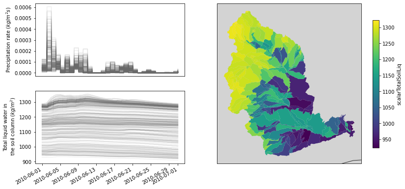
Further configuration, and more advanced parallelism

The Yakima River Basin given as an example here is a relatively small simulation of about 300 HRU for a month, but the parallelism approach built into the Distributed object can generally scale to many cores. Under the hood we rely on the `dask library <https://dask.org/>`__ to manage the scheduling of the parallel runs of both the Ensemble and Distributed objects. While we won’t actually run any simulations with these configurations, we show the code as a reference.

from dask.distributed import Client
from dask.distributed import LocalCluster
from dask_jobqueue import SLURMCluster

For local runs (e.g. your laptop or a big workstation machine), you can use the LocalCluster. For use on HPC machines, you will probably need to submit your jobs to the scheduler. This can be done via `dask_jobqueue <https://jobqueue.dask.org/en/latest/>`__. Here we show how to use the SLURMCluster, but other schedulers are supported.

# Local example
N_WORKERS = 16 # A big machine might have 16 processors
local_cluster = LocalCluster(n_workers=N_WORKERS, threads_per_worker=1) # Each SUMMA simulation runs as a single-threaded process by default
local_example = Client(local_cluster) # This connects the compute cluster to the process running in this notebook

yakima_local = ps.Distributed(summa_exe, file_manager, client=local_example)

# If you have the resources, you can just call `yakima_local.run()` just as before

# SLURM example
N_WORKERS = 285 # On HPC maybe we want to run each GRU independently
slurm_cluster = SLURMCluster(cores=N_WORKERS, memory='4GB',      # Set the number of cores and memory per worker
                             queue='default', project='Pxyzxyz') # Set your queue and project code

slurm_example = Client(slurm_cluster) # This connects the compute cluster to the process running in this notebook
yakima_slurm = ps.Distributed(summa_exe, file_manager, client=slurm_example)

# If you have the resources, you can just call `yakima_slurm.run()` just as before

Tutorial 4: Calibration of a point SUMMA simulation with Ostrich

This notebook outlines the initial work on interfacing Ostrich into the pysumma workflow. The basic workflow is similar to that of the other pysumma objects, with some initialization of an object, configuration, and finally a run call. Before digging in I’ll describe at a high level detail how the Ostrich object works. The Ostrich object basically manages the initial state of the calibration and will write out all of the necessary files to actually run the calibration. It only is a very thin wrapper around a subprocess call out to Ostrich itself. The Ostrich program will begin by setting initial parameter values and runs SUMMA through run_script.py, which is written by the Ostrich object. This run script will also handle the updating of the SUMMA parameter datastructures and evaluating the run with several metrics which can be used as loss functions. So far I have implemented KGE, MAE, and RMSE as well as a number of other helper pieces that I’ll explain later.

As usual we will begin with some standard imports and configuration, along with loading in some data that we’ll use to determine default parameters.

%pylab inline
%load_ext autoreload
%autoreload 2
%reload_ext autoreload
import pandas as pd
import pysumma as ps

veg_igbp = pd.read_csv('./VEGPARM_IGBP_MODIS_NOAH.TBL',
                       index_col=-1, skipinitialspace=True)
veg_igbp.index = veg_igbp.index.map(lambda x: x.strip().replace("'", ""))

soil_rosetta = pd.read_csv('./SOILPARM_ROSETTA.TBL',
                           index_col=-1, skipinitialspace=True)
soil_rosetta.index = soil_rosetta.index.map(lambda x: x.strip().replace("'", ""))

Populating the interactive namespace from numpy and matplotlib

Definition of the ps.Ostrich object

The ps.Ostrich object requires at least 3 inputs, along with optional specification of the python executable to use. The required arguments are: * ostrich_exe : the path to the Ostrich executable * summa_exe : the path to the SUMMA executable * file_manger : the path to the SUMMA setup file manager to calibrate * python_path : (optional) the path to the python executable that will be used to run SUMMA via pysumma.

The python_path may be necessary for you to specify because of conda/virtual environments. As usual, we define the object by instantiating it with these arguments.

site = 'BE-Bra'
summa_exe = '/pool0/data/andrbenn/summa/bin/summa.exe'
ostrich_exe = '/pool0/home/andrbenn/data/naoki_calib_example/ostrich.exe'
python_exe = '/pool0/data/andrbenn/.conda/all/bin/python'
ostrich = ps.Ostrich(ostrich_exe, summa_exe, f'./{site}/file_manager.txt', python_path=python_exe)

Configuration of the ps.Ostrich object

Before the calibration can be started we have to fill out a bit more information. The method of doing so right now is to manually assign each of the required pieces of information. Hopefully in the future we can streamline this process while allowing for ease of customization, but for now consider the interface to be in flux. The first thing that needs to be set is some information about how to calculate the objective function at each calibration step. We do this with several pieces of information, first setting the observation data file and the calibration variables in both the simulated and observed datasets. Then, you can specify a simple function to convert the observed and simulated data to match. In our case the observed data simply needs to be multiplied by negative one. Functions of this sort (lambdas) are the only supported method of conversion for the moment, and should be self contained (AKA not making any external function calls. Finally, we say that we want to calibrate using root mean square error as our objective function and that we want to minimize it (or rather, that we don’t want to maximize it). As said earlier, the cost_function can be set to one of RMSE, MAE, or KGE for the moment. If setting the cost_function to KGE then you probably want to set maximize to True.

ostrich.obs_data_file = f'/pool0/data/andrbenn/workspace/ostrich_example/{site}/forcings/{site}.nc'
ostrich.sim_calib_var = 'scalarLatHeatTotal'
ostrich.obs_calib_var = 'Qle_cor'
ostrich.import_strings = 'import numpy as np'
ostrich.conversion_function = lambda x: -x
ostrich.filter_function = lambda x: (x.isel(time=np.logical_and(x.time.dt.hour > 6, x.time.dt.hour < 20))
                                      .sel(time=slice('2009-04-01', '2010-09-30')))
ostrich.cost_function = 'KGE'
ostrich.maximize = True

Now, we set a couple of the optimization algorithm parameters and interact with the ostrich object’s internal ps.Simulation object. First, we will set the max_iters and perturb_val - these control how many calibration runs to do and how “hard” to perturb our test parameters (which will be defined later). Then we set the run times of ostrich.simulation , which is simply a pysumma Simulation object wrapped inside of the Ostrich object. We will also retrieve the local_attributes from the ostrich.simulation object, which contains the definitions of the soil and vegetation types which we will use to define our starting parameters.

ostrich.max_iters = 100
ostrich.perturb_val = 0.2
ostrich.simulation.decisions['simulStart'] = '2009-01-01 23:30'
ostrich.simulation.decisions['simulFinsh'] = '2010-10-01 23:30'
attr = ostrich.simulation.local_attributes

Setting parameters and ranges

Once we have all of that we can work on setting up our default parameters from the soil and vegetation types. To do so, we will select out the soil and vegetation parameters for our specific run from the soil and vegetation tables loaded in at the beginning of this notebook. Then, I define some rooting depths that were not included in those tables for use later. Following that, I set some initial_values that will be used in the following cell when creating the calibration parameter objects.

soil_params = soil_rosetta[soil_rosetta['SOILTYPINDEX'] == attr['soilTypeIndex'].values[0]]
veg_params = veg_igbp[veg_igbp['VEGTYPINDEX'] == attr['vegTypeIndex'].values[0]]

# Source: Zeng 2001 AMS
igbp_rooting_depths = {1: 1.8,  2: 3.0,  3: 2.0,   4: 2.0,  5: 2.4,  6: 2.5,  7: 3.10,  8: 1.7,
                       9: 2.4, 10: 1.5, 11: 0.01, 12: 1.5, 13: 1.5, 14: 1.5, 15: 0.01, 16: 4.0}

initial_values = {
    'rootingDepth': igbp_rooting_depths[attr['vegTypeIndex'].values[0]],
    'theta_res': soil_params['theta_res'].values[0],
    'theta_sat': soil_params['theta_sat'].values[0],
    'vGn_n': soil_params['vGn_n'].values[0],
    'critSoilTranspire': soil_params['REFSMC'].values[0],
    'k_soil': soil_params['k_soil'].values[0],
}

The cell following this text contains the first definition of basic calibration parameters, which are defined by OstrichParam objects. These are quite simple objects which are mainly used for converting values to the correct string template that will be used by Ostrich internally. The way that you construct a single OstrichParam is to supply the parameter name as SUMMA sees it, the starting value and a range of values that Ostrich will search within. We provide a list of these

OstrichParams to the ostrich object in the calib_params attribute.

ostrich.calib_params = [
    ps.OstrichParam('k_soil', initial_values['k_soil'], (1e-7, 0.001)),
    ps.OstrichParam('rootingDepth', initial_values['rootingDepth'], (0.01,  5.0)),
    ps.OstrichParam('theta_res', initial_values['theta_res'],   (0.001,  0.3)),
    ps.OstrichParam('theta_sat', initial_values['theta_sat'],   (0.3,   0.85)),
    ps.OstrichParam('windReductionParam', 0.50,   (0.0,   1.0)),
    ps.OstrichParam('leafDimension', 0.04, (0.01, 0.1)),
]

Of course, this basic parameter search can lead up putting you into parameter space which is not physically possible, so we need to have the ability to “tie” parameters together with some constraints. To do so, you can use the add_tied_param method on the ostrich object. Currently this only provides linear, bounded support between two other parameters, and no linked-tied parameters (that is a tied parameter can’t be used as a bound on another tied parameter). The syntax here is to

provide the tied parameter name, along with the parameter names that the tied parameter must be between. Ostrich will handle the rest from here.

ostrich.add_tied_param('fieldCapacity', lower_bound='theta_res', upper_bound='theta_sat')
ostrich.add_tied_param('critSoilTranspire', lower_bound='theta_res', upper_bound='theta_sat')

Running and viewing output

Finally, we can write the configuration and run the optimization routine. For the moment I am leaving the write and run sections separate because the API is not stable and it is often useful to just write the configurationa and inspect it manually. At some point it will likely become incorporated directly into the run method as well, but currently this is the approach we take. Neither method requires any arguments. The run of this for 10 two year runs (as we specifed several code cells earlier) will take a bit to run. Following that we will simply print the standard output. It shows the output that you would normally see during runtime of Ostrich, but more statistics and diagnostics of the calibration will be incorporated into future versions of pysumma.

ostrich.write_config()

ostrich.run()
print(ostrich.stdout)

Starting up MPI required 0.000169 seconds
--------------------------------------------------------------------------
 OSTRICH version 17.12.19 (Built Dec 19 2017 @ 12:26:43)

 A computer program for model-independent calibration and optimization.

 Author             L. Shawn Matott
 Copyright (C) 2007 L. Shawn Matott

 This program is free software; you can redistribute
 it and/or modify it under the terms of the GNU
 General Public License as published by the Free
 Software Foundation; either version 2 of the
 License, or(at your option) any later version.

 This program is distributed in the hope that it will
 be useful, but WITHOUT ANY WARRANTY; without even
 the implied warranty of MERCHANTABILITY or FITNESS
 FOR A PARTICULAR PURPOSE. See the GNU General Public
 License for more details.

 You should have received a copy of the GNU General
 Public License along with this program; if not,
 write to the Free Software Foundation, Inc., 59
 Temple Place, Suite 330, Boston, MA 02111-1307 USA
--------------------------------------------------------------------------

Ostrich Setup
Model                  : /pool0/data/andrbenn/workspace/ostrich_example/BE-Bra/calibration/run_script.py > OstExeOut.txt 2>&1
Algorithm              : Dynamically Dimensioned Search Algorithm (DDS)
Objective Function     : GCOP
Number of Parameters   : 5
Number of Tied Params  : 0
Number of Observations : 0
Seed for Random Nums.  : 42
Number of Resp. Vars        : 1
Number of Tied Resp. Vars   : 1
Number of Constraints       : 0
Penalty Method              : Additive Penalty Method (APM)

Ostrich Run Record
trial    best fitness   k_soil_mtp    rootingDepth_mtp  windReductionParam_mtp  leafDimension_mtp  summerLAI_mtp   trials remaining
1     -1.610490E-01  7.438520E-05  2.400000E+00  5.000000E-01  4.000000E-02  3.000000E+00  9.900000E+01
   1...
Operation is complete

2     -1.971280E-01  1.439891E-04  3.118226E+00  4.878725E-01  3.634539E-02  2.524366E+00  9.800000E+01

DDS is searching for a better solution.
   1...   2...
Operation is complete

4     -2.539060E-01  1.439891E-04  3.785837E+00  3.172336E-03  4.866133E-02  2.524366E+00  9.600000E+01
   3...
Operation is complete

5     -2.832170E-01  1.439891E-04  3.785837E+00  2.186533E-01  4.866133E-02  8.954278E-01  9.500000E+01

DDS is searching for a better solution.
   1...   2...
Operation is complete

7     -3.750430E-01  8.456853E-06  3.785837E+00  2.186533E-01  5.674160E-02  8.954278E-01  9.300000E+01

DDS is searching for a better solution.
   1...   2...   3...
Operation is complete

10    -3.834180E-01  8.456853E-06  3.785837E+00  1.552120E-01  9.770673E-02  8.954278E-01  9.000000E+01

DDS is searching for a better solution.
   1...   2...   3...
Operation is complete

13    -3.834180E-01  8.456853E-06  3.785837E+00  1.552120E-01  9.770673E-02  1.857542E+00  8.700000E+01
   4...
Operation is complete

14    -4.174280E-01  8.456853E-06  4.663890E+00  1.552120E-01  9.623314E-02  2.710123E+00  8.600000E+01

DDS is searching for a better solution.
   1...   2...   3...
Operation is complete

17    -4.174500E-01  8.456853E-06  4.664965E+00  1.552120E-01  9.623314E-02  2.710123E+00  8.300000E+01

DDS is searching for a better solution.
   1...   2...
Operation is complete

19    -4.506680E-01  1.865815E-04  4.664965E+00  4.455703E-01  9.623314E-02  8.730342E-01  8.100000E+01

DDS is searching for a better solution.
   1...   2...   3...
Operation is complete

22    -4.927490E-01  2.260646E-04  4.664965E+00  6.988841E-01  9.623314E-02  8.730342E-01  7.800000E+01

DDS is searching for a better solution.
   1...   2...   3...   4...   5...   6...   7...   8...   9...  10...
  11...  12...
Operation is complete

34    -4.927490E-01  2.260646E-04  4.664965E+00  6.988841E-01  9.623314E-02  1.659186E+00  6.600000E+01

DDS is searching for a better solution.
   1...   2...
Operation is complete

36    -5.012780E-01  1.428445E-04  4.664965E+00  7.456359E-01  9.623314E-02  1.659186E+00  6.400000E+01
   3...
Operation is complete

37    -5.012780E-01  1.428445E-04  4.664965E+00  7.456359E-01  9.623314E-02  6.370261E-01  6.300000E+01

DDS is searching for a better solution.
   1...   2...   3...
Operation is complete

40    -5.095020E-01  2.684462E-05  4.664965E+00  7.456359E-01  9.623314E-02  6.370261E-01  6.000000E+01

DDS is searching for a better solution.
   1...   2...   3...
Operation is complete

43    -5.248270E-01  7.023297E-06  4.664965E+00  7.456359E-01  9.623314E-02  6.370261E-01  5.700000E+01
   4...
Operation is complete

44    -5.301650E-01  7.023297E-06  4.955542E+00  7.456359E-01  9.623314E-02  1.246376E+00  5.600000E+01
   5...
Operation is complete

45    -5.301650E-01  7.023297E-06  4.955542E+00  7.456359E-01  9.623314E-02  6.007198E-01  5.500000E+01

DDS is searching for a better solution.
   1...   2...   3...
Operation is complete

48    -5.390430E-01  7.023297E-06  4.955542E+00  8.030981E-01  9.623314E-02  6.007198E-01  5.200000E+01
   4...
Operation is complete

49    -5.460650E-01  7.023297E-06  4.955542E+00  8.504111E-01  9.623314E-02  6.007198E-01  5.100000E+01

DDS is searching for a better solution.
   1...   2...
Operation is complete

51    -5.607890E-01  7.023297E-06  4.955542E+00  9.559419E-01  9.623314E-02  6.007198E-01  4.900000E+01

DDS is searching for a better solution.
   1...   2...   3...   4...
Operation is complete

55    -5.607890E-01  7.023297E-06  4.955542E+00  9.559419E-01  9.623314E-02  2.980191E+00  4.500000E+01

DDS is searching for a better solution.
   1...   2...   3...   4...
Operation is complete

59    -5.607890E-01  7.023297E-06  4.955542E+00  9.559419E-01  9.623314E-02  3.080925E+00  4.100000E+01

DDS is searching for a better solution.
   1...   2...   3...   4...
Operation is complete

63    -5.621310E-01  7.023297E-06  4.955542E+00  9.660100E-01  9.623314E-02  3.080925E+00  3.700000E+01

DDS is searching for a better solution.
   1...   2...   3...
Operation is complete

66    -5.621310E-01  7.023297E-06  4.955542E+00  9.660100E-01  9.623314E-02  3.885631E+00  3.400000E+01

DDS is searching for a better solution.
   1...   2...   3...   4...   5...
Operation is complete

71    -5.621310E-01  7.023297E-06  4.955542E+00  9.660100E-01  9.623314E-02  1.770040E+00  2.900000E+01
   6...
Operation is complete

72    -5.621310E-01  7.023297E-06  4.955542E+00  9.660100E-01  9.623314E-02  6.265755E-01  2.800000E+01

DDS is searching for a better solution.
   1...   2...
Operation is complete

74    -5.621310E-01  7.023297E-06  4.955542E+00  9.660100E-01  9.623314E-02  2.618509E+00  2.600000E+01

DDS is searching for a better solution.
   1...   2...   3...
Operation is complete

77    -5.621310E-01  7.023297E-06  4.955542E+00  9.660100E-01  9.623314E-02  1.749049E+00  2.300000E+01

DDS is searching for a better solution.
   1...   2...   3...
Operation is complete

80    -5.621310E-01  7.023297E-06  4.955542E+00  9.660100E-01  9.623314E-02  1.164108E+00  2.000000E+01
   4...
Operation is complete

81    -5.621310E-01  7.023297E-06  4.955542E+00  9.660100E-01  9.623314E-02  3.619872E+00  1.900000E+01

DDS is searching for a better solution.
   1...   2...
Operation is complete

83    -5.621310E-01  7.023297E-06  4.955542E+00  9.660100E-01  9.623314E-02  1.426859E+00  1.700000E+01

DDS is searching for a better solution.
   1...   2...
Operation is complete

85    -5.658310E-01  7.023297E-06  4.955542E+00  9.942457E-01  9.623314E-02  1.426859E+00  1.500000E+01

DDS is searching for a better solution.
   1...   2...
Operation is complete

87    -5.658310E-01  7.023297E-06  4.955542E+00  9.942457E-01  9.623314E-02  4.554346E+00  1.300000E+01

DDS is searching for a better solution.
   1...   2...   3...
Operation is complete

90    -5.658310E-01  7.023297E-06  4.955542E+00  9.942457E-01  9.623314E-02  5.749287E+00  1.000000E+01

DDS is searching for a better solution.
   1...   2...   3...   4...
Operation is complete

94    -5.658310E-01  7.023297E-06  4.955542E+00  9.942457E-01  9.623314E-02  7.144379E+00  6.000000E+00

DDS is searching for a better solution.
   1...   2...   3...   4...
Operation is complete

98    -5.658310E-01  7.023297E-06  4.955542E+00  9.942457E-01  9.623314E-02  4.982360E+00  2.000000E+00

DDS is searching for a better solution.
   1...   2...
Operation is complete

100   -5.658310E-01  7.023297E-06  4.955542E+00  9.942457E-01  9.623314E-02  4.982360E+00  0.000000E+00

Optimal Parameter Set
Objective Function : -5.658310E-01
k_soil_mtp         : 7.023297E-06
rootingDepth_mtp   : 4.955542E+00
windReductionParam_mtp : 9.942457E-01
leafDimension_mtp  : 9.623314E-02
summerLAI_mtp      : 4.982360E+00

Summary of Constraints

Algorithm Metrics
Algorithm               : Dynamically-Dimensioned Search Algorithm (DDS)
Desired Convergence Val : N/A
Actual Convergence Val  : N/A
Max Generations         : 100
Actual Generations      : 100
Peterbation Value       : 0.200000
Total Evals             : 101
Telescoping Strategy    : none
Algorithm successfully converged on a solution, however more runs may be needed
Shutting down MPI required 0.000000 seconds
Ostrich Error Report for Processor 0
A total of 1 errors and/or warnings were reported
FILE I/O ERROR             : No constraints specified.
num CTORS: 17
num DTORS: 17